In order to run WIEN2k several c-shell scripts are provided which link the individual programs to specific tasks.
All available (user-callable) commands have the ending _lapw so you can easily get a list of all commands using
ls $WIENROOT/in the directory of the WIEN2k executables. (Note: all of the more important commands have a link to a short name omitting ``_lapw''.) All these commands have at least one option, -h, which will print a small help indicating purpose and usage of this command._lapw
The main WIEN2kscript, x_lapw or x, executes a single WIEN2kprogram. First it creates the corresponding program.def-file, where the connection between Fortran I/O-units and filenames are defined. One can modify its functionality with several switches, modifying file definitions in case of spin-polarized or complex calculations or tailoring special behaviour. All options are listed with the help switch
x -h or x_lapw -h
With some of the options the corresponding input files may be changed temporarely, but are set back to the original state upon completion.
USAGE:  x PROGRAMNAME [flags]

PURPOSE:runs WIEN executables:  afminput,aim,arrows,broadening,cif2struct,
      clmaddsub,clmcopy,clminter,dipan,dstart,eosfit,eosfit6,filtvec,init_xspec,
      hex2rhomb,irrep,joint,kgen,kram,lapw0,lapw1,lapw2,lapw3,lapw5,lapw7,
      lapwdm,lapwso,lcore,lorentz,lstart,mini,mixer,nn,pairhess,plane,qtl,
      optic,optimize,orb,rhomb_in5,sgroup,spaghetti,struct_afm_check,sumpara,
      supercell,symmetry,symmetso,telnes3,tetra,txspec,xspec, dmftproj

FLAGS:
-f FILEHEAD ->  FILEHEAD for path of struct & input-files
-t/-T ->        suppress output of running time
-h/-H ->        help
-d    ->        create only the def-file
-up   ->        runs up-spin
-dn   ->        runs dn-spin
-du   ->        runs up/dn-crossterm
-sc   ->        runs semicore calculation
-c    ->        complex calculation (no inversion symmetry present)
-p    ->        run lapw1/2/so in parallel (needs .machines file)
-orb  ->        runs lapw1 with LDA+U/OP or B-ext correction
-it   ->        runs lapw1 with iterative diagonalization
-noHinv   ->    runs lapw1 with iterative diag. without  Hinv
-noHinv0  ->    runs lapw1 with iterative diag. writing new Hinv
-nohns->        runs lapw1 without HNS
-nmat_only->    runs lapw1 and yields only the matrixsize
-in1orig  ->    runs lapw2 but does not modify case.in1
-emin X ->      runs lapw2 with EMIN=X (in bin9_blaha.in2)
-all X Y ->     runs lapw2 with ALL and E-window X-Y (in bin9_blaha.in2)
-qtl  ->        calculates QTL in lapw2
-alm  ->        calculates ALM,BLM in lapw2
-almd  ->       calculates ALM,BLM in lapw2 for DMFT (Aichhorn/Georges/Biermann)
-qdmft ->       calculates charges including DMFT (Aichhorn/Georges/Biermann)
-help_files ->  creates case.helpXX files in lapw2
-vresp->        creates case.vrespval (for TAU/meta-GGA) in lapw2
-eece ->        for hybrid-functionals (lapw0,lapw2,mixer,orb,sumpara)
-grr  ->        lapw0 for grad rho/rho (using SRC.in0_grr with ixc=50)
-band ->        for bandstructures: unit 4 to 5 (in1), sets QTL and ROOT (in2)
-fermi->        calculates Fermi energy and weights in lapw2
-efg  ->        calculates lapw2 with EFG switch
-so   ->        runs lapw2 with def-file for spin-orbit calculation
-fbz   ->       runs kgen and generates a full mesh in the BZ
-fft  ->        runs dstart only up to case.in0_std creation
-super->        runs dstart and creates new_super.clmsum (and not case.clmsum)
-sel  ->        use reduced vector file in lapw7
-settol 0.000x -> run sgroup with different tolerance
-sigma->        run lstart with case.inst_sigma (autogenerated) for diff.dens.
-rxes->         run tetra using case.rxes weight file for RXES-spectroscopy.
-rxesw E1 E2->  run tetra and create case.rxes file for RXES for energies E1-E2
-delta->        run arrows program with difference between two structures
-lcore->        runs dstart with SRC.rsplcore (produces SRC.clmsc)
-copy ->        runs pairhess and copies .minpair to .minrestart and .minhess
-telnes  ->     run qtl after generating case.inq based on case.innes
USE: x -h PROGRAMNAME   for valid flags for a specific program
Note: To make use of a scratch file system, you may specify such a filesystem in the environment variable SCRATCH (it may already have been set by your system administrator). However, you have to make sure that there is enough disk-space in the SCRATCH directory to hold your case.vector* and case.help* files.
In order to start a new calculation, one should make a new subdirectory and run all calculations from there. At the beginning one must provide at least one file (see 3), namely case.struct (see 4.3) (case.inst can be created automatically on the ``fly'', see 6.4.3), then one runs a series of programs using init_lapw. This script is described briefly in chapter 4.5) and in detail in ``Getting started'' for the example TiC (see chapter 3). You can get help with switch -h. All actions of this script are logged in short in :log and in detail in the file case.dayfile, which also gives you a ``restart'' option when problems occurred. In order to run init_lapw starting from a specific point on, specify -s PROGRAM.
Ignoring ERRORS and in many cases also WARNINGS during the execution of this script, most likely will lead to errors at a later stage. Neglecting warnings about core-leakage creates .lcore, which directs the scf-cycle to peform a superposition of core densities.
init_lapw supports switch -b, a ``batch'' mode (non-interactive) for trivial cases AND experienced users. You can supply various options and specify spin-polarization, XC-potential, RKmax, k-mesh or mixing. See init_lapw -h for more details. Changes to case.struct by nn will be accepted, but by sgroup will be neglected. Please check the terminal output for ERRORS and WARNINGS !!!
In order to perform a complete SCF calculation, several types of scripts are provided with the distribution. For the specific flow of programs see chapter 4.5.
Cases with/without inversion symmetry and with/without semicore or core states are handled automatically by these scripts. All activities of these scripts are logged in short in :log (appended) and in detail together with convergence information in case.dayfile (overwriting the old ``dayfile``). You can always get help on its usage by invoking these scripts with the -h flag.
run_lapw -h
PROGRAM:        /zeus/lapw/WIEN2k/bin/run_lapw

PURPOSE:        running the nonmagnetic scf-cycle in WIEN
                to be called within the case-subdirectory
                has to be located in WIEN-executable directory

USAGE:          run_lapw [OPTIONS] [FLAGS]

OPTIONS:
-cc LIMIT ->    charge convergence LIMIT (0.0001 e)
-ec LIMIT ->    energy convergence LIMIT (0.0001 Ry)
-fc LIMIT ->    force  convergence LIMIT (1.0 mRy/a.u.)
                default is -ec 0.0001; multiple convergence tests possible
-e PROGRAM ->   exit after PROGRAM ()
-i NUMBER ->    max. NUMBER (40) of iterations
-s PROGRAM ->   start with PROGRAM ()
-r NUMBER ->    restart after NUMBER (99) iterations (rm *.broyd*)
-nohns NUMBER ->do not use HNS for NUMBER iterations
-in1new N ->    create "new" in1 file after N iter (write_in1 using scf2 info)
-ql LIMIT ->    select LIMIT (0.05) as min.charge for E-L setting in new in1
-qdmft NP ->    including DMFT from Aichhorn/Georges/Biermann running on NP proc

FLAGS:
-h/-H ->        help
-I    ->        with initialization of in2-files to "TOT"
-NI   ->        does NOT remove case.broyd*  (default: rm *.broyd* after 60 sec)
-p    ->        run k-points in parallel (needs .machine file [speed:name])
-it   ->        use iterative diagonalizations
-it1  ->        use iterative diag. with recreating H_inv (after basis change)
-it2  ->        use iterative diag. with reinitialization (after basis change)
-noHinv   ->    use iterative diag. without H_inv
-vec2pratt ->   use vec2pratt instead of vec2old for iterative diag.
-so   ->        run SCF including spin-orbit coupling
-renorm->       start with mixer and renormalize density
-in1orig->      if present, use case.in1_orig file; do not modify case.in1

CONTROL FILES:
.lcore          runs core density superposition producing case.clmsc
.stop           stop after SCF cycle
.fulldiag       force full diagonalization
.noHinv         remove case.storeHinv files
case.inm_vresp  activates calculation of vresp files for meta-GGAs
case.in0_grr    activates a second call of lapw0 (mBJ pot., or E_xc analysis)

ENVIRONMENT VARIBLES:
SCRATCH         directory  where vectors and help files should go
Additional flags valid only for magnetic cases (runsp_lapw) include:
-dm   ->        calculate the density matrix (when -so is set, but -orb is not)
-eece ->        use "exact exchange+hybrid" methods
-orb  ->        use LDA+U, OP or B-ext correction
-orbc ->        use LDA+U correction, but with constant V-matrix
Calling run_lapw (after init_lapw) from the
subdirectory case will perform up to 40 iterations (or what
you specified with switch -i) unless convergence has been reached
earlier. You can choose from three convergence criteria, -ec
(the total energy convergence is the default and is set to 0.0001 Ry
for at least 3 iterations),
-fc (magnitude of force convergence for 3 iterations, ONLY if your system has
``free'' structural parameters!) or -cc
(charge convergence, just the last iteration), and any combination
can also be specified. Be careful with these criteria,
different systems will require quite different limits (e.g. fcc Li can
be converged to ![]() Ry, a large unit cell with heavy magnetic atoms only to
0.1 mRy). You can stop the scf iterations after the current cycle
by generating an empty file .stop (use eg. touch .stop in the
respective case-directory).
Ry, a large unit cell with heavy magnetic atoms only to
0.1 mRy). You can stop the scf iterations after the current cycle
by generating an empty file .stop (use eg. touch .stop in the
respective case-directory).
The scf-cycle creates case.broyd* files which contain the "charge-history". Once run_lapw has finished, you should usually "save_lapw" (see below) the results. When you continue with another run_lapw without "save_lapw" (because the previous run did not fulfill the convergence criteria or you want to specify a more strict criterium) the "broyden-files" will be deleted unless you specify -NI.
With -e PROGRAM you can run only part of one scf cycle (e.g. run lapw0, lapw1 and lapw2), with -s PROGRAM you can start at an arbitrary point in the scf cycle (e.g. after a previous cycle has crashed and you want to continue after fixing the problem) and continue to self-consistency. Before mixer is invoked, case.clmsum is copied to case.clmsum_old, and the final ``important`` files of the scf calculation are case.clmsum and case.scf.
Invoking
run_lapw -I -i 30 -fc 0.5
will first set in case.in2 the TOT-switch (if FOR was set) to save cpu time, then run up to 30 scf cycles till the force criterion of 0.5 mRy/a.u. is met (for 3 consecutive iterations). Then the calculation of all terms of the forces is activated (setting FOR in case.in2) for a final iteration.
By default the file case.in1 is updated after lapw2 and the current Fermi-energy is inserted. This will force lapw1 to use instead of the default energy parameters (0.30) an energy ``''. The switch -in1orig can be used to keep the present case.in1 file unmodified (or to copy case.in1_orig back after -in1new).
The switch -in1new N preserves for N iteration the current case.in1 file. After the first N iterations write_in1_lapw is called and a new case.in1 file is generated, where the energy parameters are set according to the :EPLxx and :EPHxx values of the last scf iteration and the -ql value (see sections 4.4 and 7.3). In this way you may select in some cases better energy-parameters and also additional LOs to improve the linearization may be generated automatically. Note, however, that this option is potentially unsave and dangerous, since it may set energy-parameters of LOs and APW+lo too close (leading to ghostbands) or in cases where you have a ``bad'' last iteration (or large changes from one scf iteration to the next. The original case.in1 file is saved in case.in1_orig and is used as template for all further scf-cycles.
Parallelization is described in Sec. 5.5.
Iterative diagonalization, which can significantly save computer time (in particular for cases with ``few electrons'' (like surfaces) and ``large matrices (larger than 2000)'' a factor 2-5 ! is possible), is described in Sec. 7.3. It needs the case.vector.old file from the previous scf-iteration (and this file is created from case.vector when the -it switch is set) and an inverse of a previous Hamiltonian () stored in case.storeHinv. When you change the Hamiltonian significantly (changing RKmax or local orbitals), reinitialize the iterative diagonalization either by ``touch .fulldiag'' (performs one full diagonalization) or ``touch .noHinv'' (recreates case.storeHinv files) or using the -it1|-it2 switch.
You can save computer time by performing the first scf-cycles without calculating the non-spherical matrix elements in lapw1. This option can be set for N iterations with the -nohns N switch.
The presence of the file .lcore directs the script to superpose the radial core densities using dstart and generating case.clmsc. It is created automatically during init_lapw when charge-leakage warnings are ignored. This option allows to reduce the number of semi-core states, but still keeping a good charge density. Unfortunately, dstart is not parallelized and thus can be slow for big cases.
The presence of the file case.in0_grr activates a second call of
lapw0, which is necessary for modified Becke-Johnson potentials (see
Section 4.5.8) or ![]() analysis.
analysis.
If you have a previous scf-calculation and changed lattice parameters or positions (volume optimization or internal positions minimization), one could use -renorm to renormalize the density prior to the first iteration., but the recommended way is to use clmextrapol_lapw.
For magnetic systems which are difficult to converge you can use the script runfsm_lapw -m M (see section 4.5.3) for the execution of fixed-spin moment (FSM) calculations.
After self-consistency has been reached, the script
save_lapw head_of_save_filename
saves case.clmsum, case.scf, case.dmat, case.vorb and case.struct under the new name and removes the case.broyd* files. Now you are ready to modify structural parameters or input switches and rerun run_lapw, or calculate properties like charge densities (lapw5), total and partial DOS (tetra) or energy bandstructures (spaghetti).
For more complicated situations, where many parameters will be changed, we have extended save_lapw so that calculations can not only be saved under the head_of_save_filename but also a directory can be specified. If you use any of the possible switches (-a, -f, -d, -s) all input files will be saved as well (and can be restored using restore_lapw).
Options to save_lapw can be seen with
save_lapw -h
Currently the following options are supported
| -h | help |
| -a | save all input files as well |
| -f | force save_lapw to overwrite previous saves |
| -d directory | save calculation in directory specified |
| -s | silent operation (no output) |
To restore a calculation the script restore_lapw can be used. This script restores the struct, clmsum, vorb and dmat files as well as all input files. Note: The input files will only be restored when save_lapw -d was used, i.e. when you have saved a calculation in an extra directory.
After restore_lapw you can continue and either run an scf cycle (run_lapw) or recreate the scf-potential (x lapw0) and the corresponding eigenvectors (x lapw1) for further tasks (DOS, electron density,...).
Options to restore_lapw are:
| -h | help |
| -f | force restore_lapw to overwrite previous files |
| -d directory | restore calculation from directory specified |
| -s | silent operation (no output) |
| -t | only test which files would be restored |
Once a case has been completed you can clean up the directory with this command. Only the most important files (scf, clmsum, struct, input and some output files) are kept. It is very important to use this command when you have finished a case, since otherwise the large vector and helpXX files will quickly fill up all your disk space.
This script migrates a case to a remote computer (to be called within the case-dir). Needs working ssh/scp without password; local and remote case-dir must have the same name.
Call it within the desired case-dir as:
migrate_lapw [FLAGS OPTIONS] [user@]host:path/case-dir
with the following options:
-put           -> transfer of files to a remote host (default)
-get           -> transfer of files from a remote host

-all           -> the complete directory is copied
-start         -> only files to start an scf cycle are copied (default for put)
-end           -> only new files resulting from an scf cycle are copied
                  (default for get)
-save savedir  -> "save_lapw -d save_dir" is issued and only save_dir is copied

FLAGS:
-h             -> help
-clean         -> a clean_lapw is issued before copying
-r             -> files in source directory are removed after copying
-R             -> source directory (and all files) are removed after copying
-s             -> do it silent (in batch mode)
-z             -> gzip files before scp (slow network)
This script generates case.inst from a case.struct file. It is used automatically in init_lapw, if case.inst is not present. Using some options (see below) it allows to define the spin-state of all/certain atoms. Note: the label ``RMT'' is necessary in case.struct.
instgen_lapw [-h -s -up -dn -nm -ask]
   -h:   generate this message
   -s:   silent operation (do not ask)
   -up:  generates spin-up configuration for all atoms (default)
   -dn:  generates spin-dn configuration for all atoms
   -nm:  generates non-magnetic configuration for all atoms
   -ask: asks for each atom which configuration it should generate
This perl-script executes x nn and uses its output to determine the atomic sphere radii (obeying recommended ratios for H, sp-, d- and f- elements). It is called automatically within init_lapw or you may call it separately using:
setrmt_lapw case [-r X ]
where case gives the head of the case.struct file. You may specify a reduction of the RMTs by X percent in order to allow for structural optimizations. It creates case.struct_setrmt.
This script creates the input file case.int for the program tetra and allows to specifiy which partial DOS (atom, l and m) should be calculated. It was provided by Morteza Jamal (m_jamal57@yahoo.com).
You can specify interactively:
  total        (for plotting 'Total Dos')
  N            (to select atom N)
    s,p,d,...  (to select a set of PDOS for previously selected atom N)
                use labels as listed in the header of your case.qtl file)
  end          (for exit)
There is also a "batch" (non-interactive) mode:
configure_int_lapw -b total 1 tot,d,d-eg,d-t2g 2 tot,s,p end
which will prepare case.int (eg. for the TiC example) with:
tic             #Title
 -1.000   0.00250   1.200  0.003     #Emin, DE, Emax, Gauss-Broad
     8                               #Number of DOS
     0 1 total-DOS
     1 1 tot-Ti
     1 4 d-Ti
     1 5 d-eg-Ti
     1 6 d-t2g-Ti
     2 1 tot-C
     2 2 s-C
     2 3 p-C
This script searches for .running.* files within the current directory (or the directory specified with ``-d full_path_directory'') and then performs a ps command for these processes. If the specified process has not been found, it removes the corresponding .running.* file after confirmation (default) or immediately (when ``-f'' has been specified).
This script searches for .running.* files within the current directory (or the directory specified with ``-d full_path_directory'') and then kills the corresponding process after confirmation (default) or immediately (when ``-f'' has been specified). It is particular usefull for killing ``k-point parallel'' jobs.
This script extracts the critical points (CP) after a Bader analysis
(x aim (-c)) from case.outputaim. It sorts
them (according to the density), removes duplicate CPs, converts units
into
![]() and produces critical_points_ang.
and produces critical_points_ang.
It is used with: �extractaim_lapw case.outputaim
This program was contributed by:
![\framebox{
\parbox[c]{12cm}{
Hartmut Enkisch \\
Institute of Physics E1b\\...
...ilinglist. If necessary, we will communicate
the problem to the authors.}
}
}](img139.png)
It produces a plot of some quantities as function of iteration number (a maximum of 6 quantities is possible at once) from the case.scf file as specified on the commandline using analyse_lapw and GNUPLOT. This plot is updated in regular intervals.
You can call scfmonitor_lapw using:
scfmonitor_lapw [-h] [-i n] [-f case.scf] [-p] arg1 [arg2 .. arg6]
-h             	help switch
-i n            show only the last n iterations
-f scf-file     use  "scf-file"  instead of the default  "case.scf"
-p             	produces file  "scfmonitor.png"  instead of X-window plot
arg1,...        arguments to monitor (like  ":ENE"  or  ":DIS" , see analyse_lapw )
The scfmonitor can also be called directly from w2web using the "Analyse" tool.
In order to have a reasonable behavior of scfmonitor the GNUPLOT window should stay in background. This can be achieved by putting a line into your .Xdefaults file like:
gnuplot*raise: off
Note: It does not make sense to start scfmonitor before the first cycle has finished because no case.scf exists at this point.
The script analyse_lapw is usually called from scfmonitor_lapw. It "greps" from an scf-file the specified arguments and produces analyse.out.
analyse_lapw is called using:
analyse_lapw [-h] scf-file arg1 [arg2 arg3 arg4 arg5 arg6]
-h              help switch
scf-file        "scf-file"  to analyse (there's no default  "case.scf" !)
arg1,...        arguments to analyse:
                atom independend:   :ENE :DIS :FER :MMT
                atom iii dependend: :CTOiii :CUPiii :CDNiii :NTOiii :NUPiii :NDNiii
                                    :DTOiii :DUPiii :DDNiii :RTOiii :EFGiii :HFFiii
                                    :MMIiii
                vector quantities:  :FORiii[x/y/z] :POSiii[x/y/z] :FGLiii[x/y/z]
                             where     magnitude      z              z   is the default
For vector quantities like :FGLiii or :POSiii (usefull with case.scf_mini) one can
specify the respective coordinate by adding x/y/z to the corresponding labels.
grepline_lapw :label 'filename*.scf' lines_for_tail or
grepline :label 'filename*.scf' lines_for_tailyou can get a list of a quantity ``:label'' (e.g. :ENE for the total energy) from several scf files at once.
initso_lapw or
initsoand you should carefully follow the instructions and explanations of the script and the explanations for case.inso given in section 7.4.
For runfsm_lapw the sequence had to be changed and the switches -updn or -dnup forces vec2old to COPY case.vectorup tocase.vectordn (and vice versa). In the runfsm_lapw case the corresponding case.vector*.old files are generated just AFTER lapw2/lapwdm and not BEFORE lapw1. Thus after runfsm_lapw has finished, the corresponding spin-up/dn vectors are case.vector*.old and NOT case.vector*.
The switches -p -local will copy $SCRATCH/case.vector* to case.vector*. It will be done automatically when you run x lapw2 -p -qtl.
An alternative script vec2pratt_lapw was provided by L.D.Marks (l-marks@northwestern.edu) which together with SRC_vecpratt mixes the last two vectors (Pratt mixing) to generate case.vector.old. It is activatd using the -vec2pratt switch in run_lapw.
It is usually called from ``min_lapw '' after a geometry step has finished and a new struct file has been generated.
It can significantly reduce the number of scf-cycles for the new geometry step.
 [1]  VARY VOLUME with CONSTANT RATIO A:B:C
 [2]  VARY C/A RATIO with CONSTANT VOLUME (tetr and hex lattices)
 [3]  VARY C/A RATIO with CONSTANT VOLUME and B/A (orthorh lattice)
 [4]  VARY B/A RATIO with CONSTANT VOLUME and C/A (orthorh lattice)
 [5]  VARY A and C (2D-case) (tetragonal or hexagonal lattice)
 [6]  VARY A, B and C (3D-case) (orthorhombic lattice)
 [7]  VARY A, B, C and Gamma (4D-case) (monoclinic lattice)
 [8]  VARY C/A RATIO and VOLUME (2D-case) (tetr and hex lattices)
It also produces a shell-script optimize.job which looks similar to:
#!/bin/csh -f
 foreach i ( \
        tic_vol_-10.0  \
        tic_vol__-5.0  \
        tic_vol___0.0  \
        tic_vol___5.0  \
        tic_vol__10.0  \
 )
     cp  $i.struct tic.struct
 #    cp  $i.clmsum tic.clmsum
 #    x dstart
 #    run_lapw -ec 0.0001 -in1new 3  -renorm
     run_lapw -ec 0.0001
     set stat = $status
     if ($stat) then
        echo "ERROR status in" $i
        exit 1
     endif
     save_lapw  ${i}
 #    save_lapw  -f -d XXX $i
 end
You may modify this script according to your needs: use runsp_lapw or even min_lapw, or specify different convergence parameters; modify the save_lapw command and change the save-name or save into a directory to separate e.g. ``gga'' and ``lda'' results. Eventually you may activate the line `` cp $i.clmsum case.clmsum'' to use a previously saved clmsum file, e.g. from a calculation with smaller RKmax, ... and deactivate the "clmextrapol_lapw" lines, but usually the latter is so efficient that this is no longer recommended.
Note: You must have a case.clmsum file (either from init_lapw or from a previous scf calculation) in order to run optimize.job.
After execution of this script you should have a series of scf-files with energies corresponding to the modified parameters, which should allow you to find the corresponding equillibrium parameters. For the volume optimization an analysis tool is available, other tools are under development).
Using the script grepline (or the ``Analysis ![]() Analyze multiple SCF-files'' menu of w2web) you get a summary of
the total energy vs. volume (c/a). The file case.analysis can
be used in eplot_lapw
to find the minimum total energy and the equilibrium volume (c/a).
Supported equation of states include the EOS2, Murnaghan and Birch-Murnaghan EOS.
Analyze multiple SCF-files'' menu of w2web) you get a summary of
the total energy vs. volume (c/a). The file case.analysis can
be used in eplot_lapw
to find the minimum total energy and the equilibrium volume (c/a).
Supported equation of states include the EOS2, Murnaghan and Birch-Murnaghan EOS.
grepline :ENE '*.scf' 1 > case.analysis
grepline :VOL '*.scf' 1 » case.analysis
Using such strategies also higher-dimensional optimizations (e.g. c/a ratio and volume) are possible in combination with the -d option of save_lapw.
For optimization of more degrees of freedom (2-4 lattice parameters), you can use the corresponding option and for analysis of the data the script parabolfit_lapw together with the program eosfit6. It performs a non-linear least squares fit, using a parabolic fit-function in your variables and get an analytic description of your energy surface. Please note, this is only a harmonic fit (no odd or higher terms) and the description may not be very good if your parameter range is large and/or the function is quite anharmonic, or you suffer from numerical noise.
For the determination of elastic constants see the description of ELAST in sec 8.14.
This package performs a convenient 2D structure optimization (Volume and c/a, i.e. tetragonal or hexagonal spacegroups). After initialization of a case, one generates a set of structures and a job-file 2Doptimize.job using the command
set2D_lapwThis calls setup2D and you have to specify the ``order of the fit'' (stored in .fordfitcoa) and the changes in volume and c/a. The resulting 2Doptimize.job script should be adapted (eg. use min_lapw instead of run_lapw; insert switches,...) and executed. Finally
ana2D_lapwcan be executed and will analyze the results. It uses a set of case.Vconst* files (produced by 2Doptimize.job and stored also in subdirectory Vconst) and the numbvcoa file. You can modify the order of the fits in .fordfitcoa and rerun ana2D_lapw to check the sensitivity of the results with the fitting. Note: Fits of high order (and few ``data points'') may lead to artificial results due to unphysical oszillations of the fit.
You can see results for
- energy vs. c/a for each volume,
- energy vs. volume (with optimized c/a) and
- c/a vs. volume.
Optionally you can specify more cases by rerunning set2D_lapw. Specify also your ``old'' volume and c/a points again (or leave them out on purpose in case they were very bad (eg. very far from the minimum). The old results will then be taken automatically into account without recalculation (unless you modify 2Doptimize.job, see the comments at the top of this file). Thus a ``good'' strategy is to use only 3x3 points (order of fit = 3) and in a second step you add points where they are needed.
When you want to rerun such an optimization with different parameters (RKmax, k-mesh, XC-potentials) modify the top of 2Doptimize.job and set answscf=no and a new savename (eg. "_pbe_rk8_1000k").
Starting with WIEN2k_11.1 there are two possibilities to determine the equilibrium position of all individual atoms automatically (obeying the symmetry constraints of a certain space group). One can use either
At present we recommend the second (new) option, although there are cases where this scheme can be slower or may even fail to converge.
A typical sequence of commands for an optimization of the internal positions would look like:
Now you have to decide which method to use:
When using the second method we recommend you read carefully $WIENROOT/SRC_mixer/Mixer_README_4.1.pdf. Overall the method is very good for semiconductors (or well behaved metals), and allows ``tricks'' like small k-mesh or small RKMax at the beginning of the minimization and using higher accuracy only towards the end.
The following text refers (mainly) to the first method using min_lapw:
When case.scf is not present, an scf-cycle will be performed first, otherwise
the corresponding forces are extracted into case.finM and the program mini generates a
new case.struct with modified atomic positions. The previous step is saved under
case_1/2/3.... Then a new scf-cycle is executed and this loop
continues until convergence (default: forces below 2mRy/bohr) is reached.
The last iteration of each geometry step is appended to case.scf_mini,
so that this file contains the complete history of the minimization and can be used to
monitor the progress (grep :ENE *mini; or :FORxxx ...).
By default (unless switch -noex is specified), min will call the script clmextrapol_lapw after the first geometry step and try to extrapolate the charge density to the new positions. This procedure usually significantly reduces the number of scf-cycles and is thus highly recommended.
mini requires an input file case.inM (see Sec. 8.15) which is created automatically and MUST NOT be changed while min_lapw is running (except the force tolerance, which terminates the optimization).
We recommend the PORT minimization method, a reverse-communication trust-region Quasi-Newton method from the Port library, which seems to be stable, efficient and does not depend too much on the users input (DELTAs, see below with NEWT). The PORT option also uses/produces a file .min_hess, which contains the (approximate) Hessian matrix (lower-triangle Cholesky factor) If you restart a minimization with different k-points, RMT, RKmax, ... or do a similar calculation (eg. for a different volume, ...) it will be copied to .minrestart (unless -nohess is specified), so that you start with a reasonable approximation for the Hessian. The program pairhess, which calculates the first Hessian, also prints out the average Hessian eigenvalue for the symmetric, symmetry-preserving modes in mRyd/au2 as well as the minimum and maximum, and also the vibration frequencies. A list of these is given at the end of case.pairhess. Note that these are not all possible modes, but only the symmetry preserving ones. Therefore if you have prior information about the vibrations of the system you can adjust the rescaling term so the average vibration frequency is about correct. (see the description of pairhess in 9.2). (In addition there is a program eigenhess, which will analyze the Hessian after the minimization has been completed. It also prints vibrational frequencies and may give you hints about dynamical instability of your system. Some more description is given in $WIENROOT/SRC_pairhess/README and at the top of the output file case.outputeig.
When using PORT you may also want to check its progress using
grep :LABEL case.outputMwhere :LABEL is :ENE (should decrease), :GRAD (should also go down, but could sometimes also go up for some time as long as the energy still decreases), :MIN (provides a condensed summary of the progress), :WARN may indicate a problem), :DD (provides information about the step sizes and mode used). Some general explanations are:
Sometimes PORT gets "stuck" (often because of inconsistencies of energy and forces due to insufficient scf convergence or a very non-harmonic potential energy surface). A good alternative is NEW1, which is a "sophisticated" steepest-descent method with optimized step size. It can be very efficient in certain cases, but can also be rather slow when the potential energy surface is rather flat in one, but steep in another direction (eg. a weakly bound molecule on a surface, but constraining the sensitive parameters, like the bond distance of the molecule, may help).
Another alternative is NEWT, where one must set proper "DELTAs" and a "FRICTION" for each atom. Unfortunately, these DELTAs determine crucially how the minimization performs. Too small values lead to many (unnecessary) "geometry steps", while too large DELTAs can even lead to divergence (and finally to a crash). Thus you MUST control how the minimization performs. We recommend the following sequence after 2-3 geometry steps:
grep :ENE *mini
:ENE  : ********** TOTAL ENERGY IN Ry =        -2994.809124
:ENE  : ********** TOTAL ENERGY IN Ry =        -2994.813852
:ENE  : ********** TOTAL ENERGY IN Ry =        -2994.818538
Good, since the total energy is decreasing.
grep :FGL001 *mini
:FGL001:  1.ATOM                         0.000          0.000         18.219
:FGL001:  1.ATOM                         0.000          0.000         12.375
:FGL001:  1.ATOM                         0.000          0.000          7.876
Good, since the force (only a force along z is present here) is decreasing reasonably fast towards zero. You must check this for every atom in your structure.
When you detect oszillations or too small changes of the forces during geometry optimization, you will have to decrease/increase the DELTAs in case.inM and rm case.tmpM. (NOTE: You must not continue with modified DELTAs but keeping case.tmpM.) Alternatively, stop the minimization (touch .minstop and wait until the last step has finished), change case.inM and restart.
You can get help on its usage with:
min -h or min_lapw -h
PROGRAM:        min

USAGE:          min [OPTIONS]

OPTIONS:
-j JOB ->       job-file JOB (default: run_lapw -I -fc 1. -i 40 )
-noex ->        does not extrapolate the density for next geometry step
-p ->           adds -p (parallel) switch to run_lapw
-it ->          adds -it (iterative diag.) switch to run_lapw
-it1 ->         adds -it1 (it.diag. with recreating H_inv) switch to $job
-it2 ->         adds -it2 (it.diag. with reinitialization) switch to $job
-noHinv ->      adds -it -noHinv (it.diag. without H_inv) switch to $job
-sp ->          uses runsp_lapw instead of run_lapw
-nohess ->      removes .minrestart (initial Hessian) from previous minimization
-m ->           extract force-input and execute mini (without JOB) and exit
-mo ->          like -m but without copying of case.tmpM1 to case.tmpM
-h/-H ->        help
-NI ->          without initialization of minimization (eg. continue after a crash)
-i NUMBER ->    max. NUMBER (50) of structure changes
-s NUMBER ->    save_lapw after NUMBER of structure changes

CONTROL FILES:
.minstop        stop after next structure change
For instance for a spin-polarized case, which converges more difficultly, you would use:
min -j ``runsp_lapw -I -fc 1.0 -i 60''
Calculations of phonons is based on a program PHONON by K.Parlinski, which runs under MS-Windows and must be ordered separately (see http://wolf.ifj.edu.pl/phonon/ )
You would define the structure of your compound in PHONON together with a supercell of sufficient size (e.g. 64 atoms). PHONON will then generate a list of necessary displacements of the individual atoms. The resulting file case.d45 must be transfered to UNIX. Here you would run WIEN2k-scf calculations for all displacements and collect the resulting forces, which will be transfered back to PHONON (case.dat and/or case.dsy). With these force information PHONON calculates phonon at arbitrary q-vectors together with several thermodynamic properties.
Please use mainly nn to reduce equivalent atoms. sgroup might change the unitcell and than the collection of forces into the original supercell is not possible (or quite difficult).
A script run_phonon has been created. Modify it according to your needs (parallelization,....) and run all cases to selfconsistency.
Note that good force convergence is essential (at least 0.1 mRy/bohr) and if your structure has free parameters, either very good equillibrium positions must have been found before, or even better, use both, positive and negative displacements to average out any resulting error from non-equillibrium positions.
This section describes two methods for running WIEN2k on parallel computers.
One method, parallelizing k-points over processors, utilizes c-shell scripts, NFS-file system and passwordless login ((public/private keys). This method works with all standard flavors of Unix without any special requirements. The parallelization is very efficient even on heterogeneous computing environments, e.g. on heterogeneous clusters of workstations, but also on dedicated parallel computers and does NOT need large network bandwidth.
The other parallelization method, which comes new with version WIEN2k_07.3, is based on fine grained methods, MPI and SCALAPACK. It is especially useful for larger systems, if the required memory size is no longer available on a single computer or when more processors than k-points are available. It requires a fast network (at least Gb-Ethernet, better Myrinet or Infiniband) or a shared memory machine. Although not as efficient as the simple k-point parallelization, the current mpi-version has been enhanced a lot and shows very good scaling with the number of processors for most parts. In any case, the number of processors and the size of the problem (number of atoms, matrixsize due to the plane wave basis) must be compatible and typically [NMAT / sqrt(processors)] .gt. 2000 should hold.
The k-point parallelization can use a dynamic load balancing scheme and is therefore usable also on heterogeneous computing environments like networks of workstations or PCs, even if interactive users contribute to the processors' work load.
If your case is large enough, but you still have to use a few k-points, a combination of both parallelization methods is possible (always use k-point parallelism if you have more than 1 k-point).
Parts of the code are executed in parallel, namely LAPW1, LAPWSO, LAPW2, LAPWDM, and OPTIC. These are the numerically intensive parts of most calculations.
Parallelization is achieved on the k-point level by distributing subsets of the k-mesh to different processors and subsequent summation of the results. The implemented strategy can be used both on a multiprocessor architecture and on a heterogeneous (even multiplatform) network.
To make use of the k-point parallelization, make sure that your system meets the following requirements:
The command for launching a remote shell is platform dependent, and usually can be 'ssh', 'rsh' or 'remsh'. It should be specified during installation when siteconfig_lapw is executed (see chapter 11).
Fine grained MPI parallel versions are available for the programs
lapw0, lapw1, and lapw2.
This parallelization method is based on parallelization libraries, including
MPI, ScaLapack, PBlas and FFTW_2.1.5 (lapw0).
The required libraries are not included with WIEN2k.
On parallel computers, however, they are usually installed.
Otherwise, free versions of these libraries are
available![[*]](footnote.png) .
.
The parallelization affects the naming scheme of the executable programs: the fine grained parallel versions of lapw0/1/2 are called lapw0_mpi, lapw1[c]_mpi, and lapw2[c]_mpi. These programs are executed by calls to the local execution environments, as in the sequential case, by the scripts x, lapw0para, lapw1para, and lapw2para. On most computers this is done by calling mpirun and should also be configured using siteconfig_lapw.
To start the calculation in parallel, a switch must be set and an input file has to be prepared by the user.
Generation of all necessary files, starting of the processes and summation of the results is done by the appropriate scripts lapw1para, lapwsopara,lapwdmpara and lapw2para (when using -p), and parallel programs lapw0_mpi, lapw1_mpi, and lapw2_mpi (when using fine grained parallelization has been selected in the .machines file).
The following .machines file describes a simple example. We assume to have 5 computers, (alpha, ... epsilon), where epsilon has 4, and delta and gamma 2 cpus. In addition, gamma, delta and epsilon are 3 times faster than alpha and beta.:
# This is a valid .machines file
#
granularity:1
1:alpha
1:beta
3:gamma:2 delta
3:delta:1 epsilon:4
residue:delta:2
lapw0:gamma:2 delta:2 epsilon:4
To each set of processors, defined by a single line in this file, a certain number of k-points is assigned, which are computed in parallel. In each line the weight (relative speed) and computers are specified in the following form:
weight:machine_name1:number1 machine_name2:number2 ...where weight is an integer (e.g. a three times more powerful machine should have a three times higher weight). The name of the computer is machine_name[1/2/...], and the number of processors to be used on these computers are number[1/2/...]. If there is only one processor on a given computer, the :1 may be omitted. Empty lines are skipped, comment lines start with #.
Assuming there are 8 k-points to be distributed in the above example, they are distributed as follows. The computers alpha and beta get 1 each. Two processors of computer gamma and one processor of computer delta cooperate in a fine grained parallelization on the solution of 3 k-points, and one processor of computer delta plus four processors of computer epsilon cooperate on the solution of 3 k-points. If there were additional k-points, they would be calculated by the first processor (or set of processors) becoming available. With higher numbers of k-points, this method ensures dynamic load balancing. If a processor is busy doing other (e.g., interactive) work, the overall calculation will not stall, but most of its work will be done by other processors (or sets of processors using MPI). This is, however, not an implementation for fail safety: if a process does not terminate (e.g., due to shutdown of a computer) the calculation will never terminate. It is up to the user to handle with such hardware failures by modifying the .machines file and restarting the calculation at the appropriate point.
During the run of lapw1para the file .processes is generated. This file is used by lapw2para to determine which case.vector* to read.
By default lapw1para will generate approximately 3 vector-files per processor, if enough k-points are available for distribution. The factor 3 is called ``granularity'' and allows for some load balancing in heterogeneous environments. If you can be sure that load balancing is not an issue (eg. because you use a queuing-system and can be sure that you will get 100% of the cpus for your jobs) it is recommended to set
granularity:1for best performance.
On shared memory machines it is advisable to add a ``residue machine'' to calculate
the surplus (residual) k-points (given by the expression
![]() ) and rely on the operating
system's load balancing scheme. Such a ``residue machine'' is
specified as
) and rely on the operating
system's load balancing scheme. Such a ``residue machine'' is
specified as
residue:machine_name:numberin the .machines file.
Alternatively, it is also possible to distribute the remaining k-points one-by-one (and not in one junk) over all processors. The option
extrafine:1can be set in the .machines file.
When using ``iterative diagonalization'' or the $SCRATCH variable (set to a local directory), the k-point distribution must be ``fixed''. This means, the ratio (k-points / processors) must be integer (sloppy called ``commensurate'' at other places in the UG) and granularity:1 should be set.
The line
lapw0:gamma:2 delta:2 epsilon:4defines the computers used for running lapw0_mpi. In this example the 6 processors of the computers gamma, delta, and epsilon run lapw0_mpi in parallel.
If fine grained parallelization is used, each set of processors defined in the .machines file is converted to a single file .machine[1/2/...], which is used in a call to mpirun (or another parallel execution environment).
When using a queuing system (like PBS, LoadLeveler or SUN-Gridengine) one can only request the NUMBER of processors, but does not know on which nodes the job will run. Thus a ``static'' .machines file is not possible. On can write a simple shell script, which will generate this file on the fly once the job has been started and the nodes are assigned to this job. Examples can be found at our web-site ``http://www.wien2k.at/reg_users/faq''.
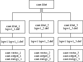
In the setup of the k-point parallel version of LAPW1 the list of k-points in case.klist (Note, that the k-list from case.in1 cannot be used for parallel calculations) is split into subsets according to the weights specified in the .machines file:
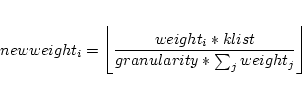
where ![]() is the number of k-points to be calculated on processor i.
is the number of k-points to be calculated on processor i.
![]() is always set to a value greater equal one.
is always set to a value greater equal one.
A loop over all ![]() processors is repeated until all k-points have been
processed.
processors is repeated until all k-points have been
processed.
Speedup in a parallel program is intrinsically dependent on the serial or
parallel parts of the code according to Amdahl's law:
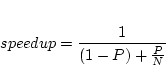
In WIEN2k usually only a small part of time is spent in the
programs lapw0, lcore and mixer which is
very small (negligible) in comparison to the times spent in
lapw1 and lapw2.
The time for waiting until
all parallel lapw1 and lapw2 processes have finished is important too.
For a good performance it is therefore necessary to have a good load balancing by
estimating properly the speed and availability of the machines used. We
encourage the use of testpara_lapw or ``Utils.
![]() testpara'' from w2web to check the
k-point distribution over the machines before actually running
the programs in parallel.
testpara'' from w2web to check the
k-point distribution over the machines before actually running
the programs in parallel.
While running lapw1 and lapw2 in parallel mode, the scripts testpara1_lapw (see 5.2.14) and testpara2_lapw (see 5.2.15) can be used to monitor the succession of parallel execution.
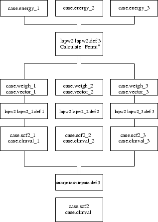
To see how files are handled by the scripts lapw1para and lapw2para refer to figures 5.1 and 5.2. After the lapw2 calculations are completed the densities and the informations from the case.scf2_x files are summarized by sumpara.
Note: parallel lapw2 and sumpara take two command line arguments, namely the case.def file but also a number_of_processor indicator.
The following parallel programs use different parallelization strategies:
Let us assume, for example, 64 processors. In a given processing step, one of these processors has to communicate with the other 63 processors if a one-dimensional setup was chosen. In the case of a two-dimensional processor setup it is usually sufficient to communicate with the processors of the same processor row (7) or the same processor column (7), i.e. with 14 processors.
In general the processor array ![]() is chosen as follows:
is chosen as follows:
![]() ,
,
 . Because of SCALAPACK, often
 ![]() arrays (i.e. 4, 9, 16,... processors) give best performance and of course
it is not recommended to use eg. 17 processors.
arrays (i.e. 4, 9, 16,... processors) give best performance and of course
it is not recommended to use eg. 17 processors.
In addition the density calculation for each atom can be further parallelized by distributing the eigenvector on a certain subset of processors (ususlly 2-4). This is not so efficient, but most usefull if the memory requirement is too big otherwise. You set it in .machines using
lapw2_vector_split:2
If more than one k-point is distributed at once to lapw1_mpi or lapw2_mpi, these will be treated consecutively.
Depending on the parallel computer system and the problem size, speedups will vary to some extend. Matrix setup in lapw1 should scale nearly perfect, while diagonalization (using SCALAPACK) will not. Usually, ``iterative'' scales better than ``full'' diagonalization and is preferred for large scale computations. Scalability over atoms will be very good if processor and atom numbers are compatible. Running the fine grained parallelization over a 100Mbit/s Ethernet network is not recommended, even for large problem sizes.
help_lapw
which opens the pdf-version of the users guide (using acroread or what
is defined in $PDFREADER).
You can search for a specific keyword using ``![]() f
keyword''. This procedure substitutes an ``Index'' and should make
it possible to find a specific information without reading through the
complete users guide.
f
keyword''. This procedure substitutes an ``Index'' and should make
it possible to find a specific information without reading through the
complete users guide.
We have included a few ``interface scripts'' into the current WIEN2k distribution, to simplify the previewing of results. In order to use these scripts the public domain program ``gnuplot'' has to be installed on your system.
The script eplot_lapw plots total energy vs. volume or total
energy vs. c/a-ratio using the file case.analysis. The latter should
have been created with grepline (using :VOL and :ENE labels) or the ``Analysis
![]() Analyze multiple SCF-files'' menu of w2web and the file
names must be generated (or compatible) with ``optimize.job''.
Analyze multiple SCF-files'' menu of w2web and the file
names must be generated (or compatible) with ``optimize.job''.
For a description of how to use the script for batch like execution call the script using
eplot_lapw -h
The script parabolfit_lapw is an interface for a harmonic fitting of E vs. 2-4-dim lattice parameters by a non-linear least squares fit (eosfit6) using PORT routines. Once you have several scf calculations at different lattice parameters (usually generated with optimize.job) it generates the required case.ene and case.latparam from your scf files. Using
parabolfit_lapw [ -t 2/3/4 ] [ -f FILEHEAD ] [ -scf '*xxx*.scf' ]
you can optionally specify the dimensionality of the fit or the specific scf-filenames.
The script dosplot_lapw plots total or partial Density of States depending on the input used by case.int and the interactive input. A more advanced plotting interface is provided by dosplot2_lapw, see below.
For a description of how to use the script for batch like execution call the script using
dosplot_lapw -h
The script dosplot2_lapw plots total or partial Density of States depending on the input used by case.int and the interactive input. It can plot up to 4 DOS curves into one plot, and simultaneously plot spin-up/dn DOS.
It was provided by Morteza Jamal (m_jamal57@yahoo.com).
For a description of how to use the script for batch like execution call the script using
dosplot2_lapw -h
The script Curve_lapw plots x,y data from a file specified interactively. It asks for additional interactive input. It can plot up to 4 curves into one plot and is a simple gnuplot interface.
It was provided by Morteza Jamal (m_jamal57@yahoo.com).
specplot_lapw provides an interface for plotting X-ray spectra from the output of the xspec or txspec program.
For a description of how to use the script for batch like execution call the script using
specplot_lapw -h
The script rhoplot_lapw produces a surface plot of the electron density from the file case.rho created by lapw5.
Note: To use this script you must have installed the C-program reformat supplied in SRC_reformat.
The script opticplot_lapw produces XY plots from the output files of the optics package using the case.joint, case.epsilon, case.eloss, case.sumrules or case.sigmak. For a description of how to use the script for batch like execution call the script using
opticplot_lapw -h
The script addjoint-updn_lapw adds the files case.jointup and case.jointdn together and produces case.joint. It uses internally the program add_columns. It should be called for spin-polarized optics calculations after x joint -up and x joint -dn, because the Kramers-Kronig transformation to the real part of the dielectric function () is not a simple additive quantity concerning the spin (see Ambrosch-Draxl 06). The KK transformation should then be done non-spinpolarized (x kram) resulting in files: case.epsilon, case.eloss, case.sumrules or case.sigmak.