In sections 7.1-7.9 we describe the main programs to run an SCF cycle as illustrated in figure 4.1.
lapw0 computes the total potential ![]() as the sum of the Coulomb
as the sum of the Coulomb
![]() and the exchange-correlation potential
and the exchange-correlation potential ![]() using the total
electron (spin) density as input. It generates the spherical part
(l=0) as case.vsp and the non-spherical part as
case.vns. For spin-polarized systems, the spin-densities
case.clmup and case.clmdn lead to two pairs of potential
files. These files are called: case.vspup, case.vnsup
and case.vspdn, case.vnsdn.
using the total
electron (spin) density as input. It generates the spherical part
(l=0) as case.vsp and the non-spherical part as
case.vns. For spin-polarized systems, the spin-densities
case.clmup and case.clmdn lead to two pairs of potential
files. These files are called: case.vspup, case.vnsup
and case.vspdn, case.vnsdn.
The Coulomb potential is calculated by the multipolar Fourier
expansion introduced by Weinert (81). Utilizing the spatial
partitioning of the unit cell and the dual representation of the
charge density [equ. 2.10], firstly the multipole
moments inside the spheres are calculated (Q-sp). The Fourier series
of the charge density in the interstitial also represent SOME density
inside the spheres, but certainly NOT the correct density there.
Nevertheless, the multipole moments of this artificial plane-wave
density inside each sphere are also calculated (Q-pw). By subtracting
Q-pw from Q-sp one obtains pseudo-multipole moments Q. Next a new
plane-wave series is generated which has two properties, namely zero
density in the interstitial region and a charge distribution inside
the spheres that reproduces the pseudo-multipole moments Q. This
series is added to the original interstitial Fourier series for the
density to form a new series which has two desirable properties: it
simultaneously represents the interstitial charge density AND it has
the same multipole moments inside the spheres as the actual density.
Using this Fourier series the interstitial Coulomb potential follows
immediately by dividing the Fourier coefficients by ![]() (up to a
constant).
(up to a
constant).
Inside the spheres the Coulomb potential is obtained by a straightforward classical Green's function method for the solution of the boundary value problem.
The exchange-correlation potential is computed numerically on a grid. Inside the atomic spheres a least squares procedure is used to reproduce the potential using a lattice harmonics representation (the linear equations are solved with modified LINPACK routines). In the interstitial region a 3-dimensional fast Fourier transformation (FFT) is used.
The total potential ![]() is obtained by summation of the Coulomb
is obtained by summation of the Coulomb ![]() and exchange-correlation potentials
and exchange-correlation potentials ![]() .
.
In order to find the contribution from the plane wave representation to the Hamilton matrix elements we reanalyze the Fourier series in such a way that the new series represents a potential which is zero inside the spheres but keeps the original value in the interstitial region and this series is put into case.vns.
The contribution to the total energy which involves integrals of the
form ![]() is calculated according to the formalism of Weinert et
al (82).
is calculated according to the formalism of Weinert et
al (82).
The Hellmann-Feynman force contribution to the total force is also calculated (Yu et al 91).
Finally, the electric field gradient (EFG) is calculated in case you have an L=2 term in the density expansion. The EFG tensor is given in both, the ``local-rotation-matrix'' coordinate system, and then diagonalized. The resulting eigenvectors of this rotation are given by columns.
For surface calculations the total and electrostatic potential at z=0 and z=0.5 is calculated and can be used as energy-zero for the determination of the workfunction. (It is assumed that the middle of your vacuum region is either at z=0 or z=0.5).
The program lapw0 is executed by invoking the command:
lapw0 lapw0.def or x lapw0 [ -p -eece -grr]
The following parameters are used (they are collected in file param.inc, but usually need not to be changed:
| NCOM | number of lm components in charge density and potential
representation; it must satisfy the following condition:
NCOM+3 .gt. |
| NRAD | number of radial mesh points |
| LMAX2 | highest L in the LM expansion of charge and potential |
| LMAX2X | highest L for the gpoint-grid in the xcpot generation (may need large values for ``-eece'') |
| restrict_output | for mpi-jobs, limits the number of case.output0xxx files to ``restrict_output'' |
The input is very simple. It is generated automatically by init_lapw, and needs to be changed only if a different exchange-correlation potential should be used:
------------------ top of file: case.in0 --------------------
TOT   13             ! MULT/COUL/EXCH/POT /TOT ;  VXC-SWITCH
NR2V      IFFT  8    ! R2V  EECE/HYBR IFFT  LUSE
 30  30 108  4.00  1 ! min IFFT-parameters, enhancement factor, iprint
0 0.0     (#of FK in E-field expansion, EFELD (Ry)

------------------- bottom of file ---------------------------
Interpretive comments follow:
| switch | ||
| TOT | total energy contributions and total potential calculated | |
| KXC | total energy contributions and total potential calculated. In addition the kinetic energy contribution as well as the XC-energy will be printed. | |
| POT | total potential is calculated, but not the total energy | |
| MULT | multipole moments calculated only | |
| COUL | Coulomb potential calculated only | |
| EXCH | exchange correlation potential calculated only | |
| NOTE: MULT, COUL, and EXCH are for testing only, whereas POT, saves some CPU time if total energy is not needed | ||
| indxc | index to specify type of exchange and correlation potential. Supported options (for more options see the SRC_lapw0/vxclm2.f subroutine) include: | |
| 5 | Perdew and Wang 92, reparameterization of Ceperly-Alder data, the recommended LDA option | |
| 13 | Generalized Gradient approximation (PBE, Perdew-Burke-Ernzerhof 96) | |
| 11 | Generalized Gradient approximation (Wu-Cohen 2006, Tran et al. 2007) | |
| 19 | Generalized Gradient approximation (PBEsol, Perdew 2008) | |
| 20 | Generalized Gradient approximation (AM05, Mattsson 2008) | |
| 12 | Meta-GGA PKZB (Perdew et al. 1999). In order to generate the requiered case.vresp* files, you need case.inm_vresp (cp $WIENROOT/SRC_templates/case.inm_vresp case.inm_vresp and run one scf cycle with PBE (indxc=13) after creation of case.inm_vresp. Only afterwards change indxc to 12. In addition you must use very large IFFT parameters, otherwise it might be numerically unstable. | |
| 27 | Meta-GGA TPSS (Tao et al. 2003). At present the ``best''
meta-GGA. (See also the option above.) Note: Only |
|
| 28 | modified Becke-Johnson (mBJ-LDA) potential |
|
| 50 | calculates the average of over the unit cell. This is used for the mBJ potential mentioned above. |
| RPRINT | NR2V | no additional output |
| R2V | Exchange-correlation (case.r2v), Coulomb
(case.vcoul) and
total potentials (case.vtotal)
are written as ( |
|
| H-mod | EECE | On-site Hartree-Fock (inside spheres) for selected electrons (see 4.5.7) |
| HYBR | On-site Hybrid functionals (inside spheres) (see 4.5.7) | |
| FFTopt | IFFT | optional keyword, which lets you define the IFFTx mesh and an enhancement factor in the next line (necessary for runeece_lapw) |
| LUSE | optional l-max value for the angular grid used in xcpot1. For standard LDA/GGA the recommended value is max L value of LM-list in case.in2 + 2; for EECE one should use a better, antialiased grid, thus a large negative LUSE-value is recommended (and set automatically by runeece_lapw) |
| IFFTx,y,z | FFT-mesh parameters in x,y,z directions for the calculation of the XC-potential in the interstitial region. Usually set automatically in init_lapw (dstart). The ratio of the 3 numbers should be indirect proportional to the lattice parameters. (-1 -1 -1 determines these numbers automatically and takes only IFFTfactor into account) | |
| IFFTfactor | Multiplicative factor to the IFFT grid specified above. It needs to be enlarged for highly accurate GGA or meta-GGA calculations as well as for systems with H atoms with small spheres. | |
| iprint | optional print switch. iprint=0 will greatly reduce case.output0 (in particular for lapw0_mpi). |
The following line is optional and can be omitted. It is used to introduce an electric field via a zig-zag potential (see J.Stahn et al. 2001):
| IFIELD | number of Fourier coefficients to model the zig-zag potential. Typically use IEFIELD=30; -999 lists available modes (form) of fields, and these modes can be specified by mode=IEFIELD/1000. (default: mode=0) | |
| EFIELD | value (amplitude) of the electric field. The electric field (in Ry/bohr) corresponds to EFIELD/c, where c is your c lattice parameter. | |
| WFIELD | optional value for lambda (see output of IEFIELD=-999). |
This program was contributed by:
![\framebox{
\parbox[c]{12cm}{
P.Nov\'ak \\
Inst. of Physics, Acad.Science, P...
...ilinglist. If necessary, we will communicate
the problem to the authors.}
}
}](img181.png)
orb calculates the orbital dependent potentials, i.e. potentials which are nonzero in the atomic spheres only and depend
on the orbital state numbers ![]() . In the present version the potential
is assumed to be independent of the radius vector and needs the density matrix calculated
in lapwdm. Four different potentials
are implemented in this package:
. In the present version the potential
is assumed to be independent of the radius vector and needs the density matrix calculated
in lapwdm. Four different potentials
are implemented in this package:
 |
(11) |
 |
(12) |
In all cases the resulting potential for a given atom and orbital number ![]() is a
Hermitian,
is a
Hermitian, ![]() x
x![]() matrix. In general this matrix is complex, but in special
cases it may be real.
matrix. In general this matrix is complex, but in special
cases it may be real.
For more information see also section 4.5.6.
The program orb is executed by invoking the command:
x orb [ -up/-dn/-du ] or orb up/dnorb.def
The following parameters are used (collected in file param.inc):
| LABC | highest l+1 value of orbital dependent potentials |
| NRAD | number of radial mesh points |
Since this program can handle three different cases, examples and descriptions of case.inorb for all cases are given below:
| nmod | defines the type of potential 1...LDA+U, 2...OP, 3... |
|
| natorb | number of atoms for which orbital potential |
|
| ipr | printing option, the larger ipr, the longer the output |
| mixmod | PRATT or BROYD (should not be changed, see MIXER for more information) | |
| amix | coefficient for the Pratt mixing of |
|
| This option is now only used for testing. The mixing should be set to PRATT, 1.0 |
| iatom | index of atom in struct file | |
| nlorb | number of orbital moments for which Vorb shall be applied | |
| lorb | orbital numbers (repeated nlorb-times) |
| nsic | defines 'double counting correction' | |
| nsic=0 | 'AMF method' (Czyzyk et al. 1994) | |
| nsic=1 | 'SIC method' (Anisimov et al. 1993, Liechtenstein et al. 1995) | |
| nsic=2 | 'HMF method' (Anisimov et al. 1991) |
| U(li,i), J(li,i) | Coulomb and exchange parameters, U and J, for LDA+U in Ry for
atom type i and orbital number li. We recommend to use
|
Example of the input file for NiO (LDA+U included for two inequivalent Ni atoms that have indexes 1 and 2 in the structure file):
---------------- top of file: case.inorb --------------------
1  2  0                        nmod, natorb, ipr
PRATT,1.0                      mixmod, amix
1 1 2                          iatom nlorb, lorb
2 1 2                          iatom nlorb, lorb
1                              nsic (LDA+U(SIC) used)
0.52 0.0                       U J
0.52 0.0                       U J
---------------- bottom of file:  --------------------
| nmodop | defines mode of 'OP' | |
| 1 | average |
|
| 0 | average |
| Ncalc(i) | ||
| 1 | Orb.pol. parameters are calculated ab-initio | |
| 0 | Orb.pol. parameters are read from input |
| pop(li,i) | OP parameter in Ry |
| direction of magnetization expressed in terms of lattice vectors |
Example of the input file for NiO (total ![]() used in (1),
OP parameters calculated ab-initio,
used in (1),
OP parameters calculated ab-initio, ![]() along [001]):
along [001]):
---------------- top of file: case.inorb --------------------
2  2  0                        nmod, natorb, ipr
PRATT, 1.0                     mixmod, amix
1 1 2                          iatom nlorb, lorb
2 1 2                          iatom nlorb, lorb
0                              nmodop
1                              Ncalc
1                              Ncalc
0. 0. 1.                       direction of M in terms of lattice vectors
---------------- bottom of file --------------------
| external field in Tesla |
| direction of magnetization expressed in terms of lattice vectors |
Example of the input file for NiO,
(![]() = 4 T, along [001]):
= 4 T, along [001]):
---------------- top of file: case.inorb --------------------
3  2  0                        nmod, natorb, ipr
PRATT, 1.0                     mixmod, amix
1 1 2                          iatom nlorb, lorb
2 1 2                          iatom nlorb, lorb
4.                             Bext in T
0. 0. 1.                       direction of Bext in terms of lattice vectors
---------------- bottom of file --------------------
lapw1 sets up the Hamiltonian and the overlap matrix (Koelling and Arbman 75) and finds by diagonalization eigenvalues and eigenvectors which are written to case.vector. Besides the standard LAPW basis set, also the APW+lo method (see Sjöstedt et al 2000, Madsen et al. 2001) is supported and the basis sets can be mixed for maximal efficiency. If the file case.vns exists (i.e. non-spherical terms in the potential), a full-potential calculation is performed.
For structures without inversion symmetry, where the hamilton and overlap matrix elements are complex numbers, the corresponding program version lapw1c must be used in connection with lapw2c.
Since usually the diagonalization is the most time consuming part of the calculations, two options exist here. In WIEN2k we include highly optimized modifications of LAPACK routines. We call all these routines ``full diagonalization'', but we also provide an option to do an ``iterative diagonalization'' using a new preconditioning of a block-Davidson method (see Singh 89 and Blaha et al. 09). The scheme uses an old eigenvector from the previous scf-iteration, and produces approximate (but usually still highly accurate) eigenvalues/vectors. The preconditioner (inverse of can be calculated at the first iterative step (which will therefore take longer than subsequent iterative steps), stored on disk (case.storeHinv) and reused in all subsequent scf-iterations (until the next ``full'' diagonalization or when it is recreated (x lapw1 -it -noHinv0)). Usually this is the fastest scheme, but storage of case.storeHinv can be large (and slow when you have a slow network) and when the Hamiltonian changes too much, performance may degrade. Alternatively, the preconditioner can be recalculated all the time (x lapw1 -it -noHinv). Depending on the ratio of matrix size to number of eigenvalues (cpu time increases linearly with the number of eigenvalues, but a sufficiently large number is necessary to ensure convergence) a significant speedup compared to ``full'' diagonalization (LAPACK) can be reached. Iterative diagonalization is activated with the -it switch in x lapw1 -it or run_lapw -it. Often the preconditioner is so efficient, that it does not need to be recalculated, even within a structural optimization and one can use min_lapw -j ``run_lapw -I -fc 1 -it''. In some cases it is preferable to use min_lapw -j ``run_lapw -I -fc 1 -it1'', which will recreate case.storeHinv, or do not store these files at all using min_lapw -j ``run_lapw -I -fc 1 -it -noHinv ''
Parallel execution (fine grain and on the k-point level) is also possible and is described in detail in Sec. 5.5.
The switch -nohns skips the calculation of the nonspherical matrix elements inside the sphere. This may be used to save computer time during the first scf cycles.
The program lapw1 is executed by invoking the command:
x lapw1 [-c -up|dn -it -noHinv|-noHinv0 -p -nohns -orb -band -nmat_only] or
lapw1 lapw1.def or lapw1c lapw1.def
In cases without inversion symmetry, the default input filename is case.in1c. For 2-window (not recommended) semi-core calculations the lapw1s.def file uses a case.in1s file and creates the files case.output1s and case.vectors. For the spin-polarized case lapw1 is called twice with uplapw1.def and dnlapw1.def. To all relevant files the keywords ``up`` or ``dn`` are appended (see the fcc Ni test case in the WIEN2k package).
The following parameters (collected in file param.inc_r or param.inc_c) are used:
| LMAX | highest l+1 in basis function inside sphere (consistent with input in case.in1) |
| LMMX | number of LM terms in potential (should be at least NCOM-1) |
| LOMAX | highest l for local orbital basis (consistent with input in case.in1) |
| NGAU | number of Gaunt coefficients for the non-spherical contributions to the matrix elements |
| NMATMAX | maximum size of H,S-matrix (defines size of program, should be chosen according to the memory of your hardware, see chapter 11.2.2!) |
| NRAD | number of radial mesh points |
| NSLMAX | highest l+1 in basis functions for non-muffin-tin matrix elements (consistent with input in case.in1).If set larger than 5, parameter MAXDIM (modules.F) and LOMAX=8, P(10,10) (gaunt2.f) must also be increased. |
| NSYM | order of point group |
| NUME | maximum number of energy eigenvalues per k-point |
| NVEC1 | defines the largest triple of integers which define reciprocal |
| NVEC2 | K-vectors when multiplied with the reciprocal Bravais matrix |
| NVEC3 | |
| NLOAT | max number of LOs for one |
| restrict_output | for mpi-jobs, limits the number of case.output1_X_proc_XXX files to ``restrict_output'' |
Below a sample input is shown for ![]() (rutile), one of the
test cases provided in the WIEN2k package. The input file is
written automatically by LSTART, but was modified to set APW only for Ti-3d
and O-2p orbitals.
(rutile), one of the
test cases provided in the WIEN2k package. The input file is
written automatically by LSTART, but was modified to set APW only for Ti-3d
and O-2p orbitals.
------------------ top of file: case.in1 --------------------
WFFIL  EF=0.5000   (WFPRI,WFFIL,SUPWF ; wave fct. print,file,suppress
  7.500   10    4  (R-mt*K-max; MAX l, max l for hns )
  0.30    5 0 (global energy parameter E(l), with 5 other choices,   LAPW)
 0   -3.00      0.020 CONT 0   ENERGY PARAMETER for s,               LAPW
 0    0.30      0.000 CONT 0   ENERGY PARAMETER for s-local orbital, LAPW-LO
 1   -1.90      0.020 CONT 0   ENERGY PARAMETER for p                LAPW
 1    0.30      0.000 CONT 0   ENERGY PARAMETER for p-local orbitals LAPW-LO
 2    0.20      0.020 CONT 1                                         APW
  0.20    3 0 (global energy parameter E(l), with 1 other choice,    LAPW)
 0   -0.90      0.020 STOP 0                                         LAPW
 0    0.30      0.000 CONT 0                                         LAPW-LO
 1    0.30      0.000 CONT 1                                         APW
K-VECTORS FROM UNIT:4   -9.0       2.0    69   emin/emax/nband
1.d-15    0.0                    spro_limit for it.diag., lambda for it.diag
------------------- bottom of file ------------------------
Interpretive comments follow:
| switch | WFFIL | standard option, writes wave functions to file case.vector (needed in lapw2) |
| SUPWF | suppresses wave function calculation (faster for testing eigenvalues only) | |
| WFPRI | prints eigenvectors to case.output1 and writes case.vector (produces long outputs!) | |
| EF | optional input. If ``EF='' key is present, lapw1 reads EF and sets all default energy parameters (0.3) to ``EF-0.2'' Ry. |
| rkmax |
|
|
| Note, that the actual matrix size is written on case.scf1. It is determined by whatever is smaller, the plane wave cut-off (specified with RKmax) or the maximum matrix dimension NMATMAX, (see previous section). | ||
| lmax | maximum l value for partial waves used inside atomic spheres (should be between 8 and 12) | |
| lnsmax | maximum l value for partial waves used in the computation of non-muffin-tin matrix elements (lnsmax=4 is quite good) |
| Etrial | default energy used for all |
|
| ndiff | number of exceptions (specified in the next ndiff lines) | |
| Napw | 0 ... use LAPW basis, 1 ... use APW-basis for all ``global'' |
| l | l of partial wave | |
| El | ||
| de | energy increment | |
| de=0: this E(l) overwrites the default energy (from line 3) | ||
| de |
||
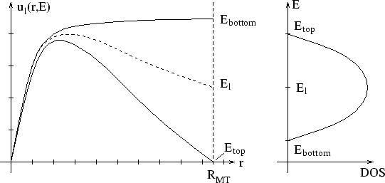
| At the bottom of the energy bands u has a zero slope
(bonding state), but it has a zero value (antibonding state)
at the top of the bands. One can search up and down in
energy starting with |
||
| switch | used only if de.ne.0 | |
| CONT | calculation continues, even if either |
|
| STOP | calculation stops if not both |
|
| NAPWL | 0 ... use LAPW basis, 1 ... use APW-basis for this |
| unit-number | file number from which the k-vectors in the irreducible wedge of the Brillouin zone are read. Default is 4, for which the corresponding information is contained in case.klist (generated by KGEN). Should not be changed. | |
| EMIN, EMAX | energy window in which eigenvalues shall be searched (overrides setting in case.klist. A small window saves computer time, but it also limits the energy range for the DOS calculation of unoccupied states. | |
| nband | number of eigenvalues calculated with iterative diagonalization. Set automatically to in lstart. Larger values will lead to more cpu-time. (Optional input) |
| spro_limit | limit for detection of linear dependency for iterative diagonalization (optional input), typical around 1.d-15) | |
| lambda_iter | optional value for preconditioner of iterative diagonalization (see above). By default we use , but in some cases convergence can be improved by a small (around 1.0) positive or negative |
| name | name of k-vector (optional) | |
| ix,iy,iz, idv | defines the k-vector, where x= ix/idv etc. We use carthesian coordinates in units
of |
|
| weight | of k-vector (order of group of k) |
lapwso includes spin-orbit (SO) coupling in a second-variational
procedure and computes eigenvalues and eigenvectors (stored in
case.vectorso) using the scalar-relativistic wavefunctions from
lapw1. For reference see Singh 94 and Novák 97. The SO
coupling must be small, as it is diagonalized in the space of the
scalar relativistic eigenstates. For large spin orbit effects it
might be necessary to include many more eigenstates from lapw1
by increasing EMAX in case.in1 (up to 10 Ry!).
We also provide an additional basisfunction, namely an LO with a ![]() radial wavefunction, which improves the basis and removes to a large degree
the dependency of the results on EMAX and RMT (see Kuneš et al. 2001).
SO is considered only within the atomic spheres and thus the results may
depend to some extent on the choice of atomic spheres radii. The nonspherical
potential is neglected when calculating
radial wavefunction, which improves the basis and removes to a large degree
the dependency of the results on EMAX and RMT (see Kuneš et al. 2001).
SO is considered only within the atomic spheres and thus the results may
depend to some extent on the choice of atomic spheres radii. The nonspherical
potential is neglected when calculating ![]() .
Orbital dependend potentials (LDA+U, EECE or OP) can be added to the hamiltonian
in a cheap and simple way.
.
Orbital dependend potentials (LDA+U, EECE or OP) can be added to the hamiltonian
in a cheap and simple way.
In spin-polarized calculations the presence of spin-orbit coupling may reduce symmetry and even split equivalent atoms into non-equivalent ones. It is then necessary to consider a larger part of the Brillouin zone and the input for lapw2 should also be modified since the potential has lower symmetry than in the non-relativistic case. The following inputs may change:
We recommend to use initso (see Sec.5.2.17) which helps you together with symmetso (see Sec.9.1) to setup spinorbit calculations.
Note: SO eigenvectors are complex and thus lapw2c must be used in a selfconsistent calculation.
The program lapwso is executed by invoking the command:
x lapwso [ -up -p -c -orb] or
lapwso lapwso.def
where here -up indicates a spin-polarized calculation (no ``-dn'' is needed, since spin-orbit will mix spin-up and dn states in one calculation).
The following parameters are used (collected in file param.inc):
| FLMAX | constant = 3 |
| LMAX | highest l of wave function inside sphere (consistent with lapw1) |
| LABC | highest l of wave function inside sphere where SO is considered |
| LOMAX | max l for local orbital basis |
| NRAD | number of radial mesh points |
| NLOAT | number of local orbitals |
A sample input for lapwso is given below. It will be generated automatically by initso
------------------ top of file: case.inso --------------------
WFFIL
 4  0  0                      llmax,ipr,kpot
 -10.0000   1.5000           Emin, Emax
     0 0 1                       h,k,l (direction of magnetization)
   2                             number of atoms with RLO
 1    -3.5      0.005 STOP       atom-number, E-param for RLO
 3    -4.5      0.005 STOP       atom-number, E-param for RLO
 1   2                           number of atoms without SO, atomnumbers
------------------- bottom of file ------------------------
Interpretive comments on this file are as follows:
| WFFIL | wavefunctions will also be calculated for scf-calculation. Otherwise only eigenvalues are calculated. |
| LLMAX | maximum l for wavefunctions | |
| IPR | print switch, larger numbers give additional output. | |
| KPOT | 0 | V(dn) potential is used for |
| 1 | averaged potential used for all matrix elements. |
| Emin | minimum energy for which the output eigenvectors and eigenenergies will be printed (Ry) | |
| Emax | maximum energy |
| h,k,l | vector describing the direction of magnetization. For R lattice use h,k,l in rhombohedral coordinates (not in hexagonal) |
| nlr | number of atoms for which a |
| nlri | atom-number for which RLO should be added | |
| El | ||
| de | energy increment (see lapw1) | |
| switch | used only if de.ne.0 | |
| CONT | calculation continues, even if either |
|
| STOP | calculation stops if not both |
| noff | number of atoms for which SO is switched off (for ``light'' elements, saves time) | |
| iatoff | atom-numbers |
lapw2 uses the files case.energy and case.vector and computes the Fermi-energy
(for a semiconductor ![]() is set to the valence band maximum)
and the expansions of the electronic charge densities in a
representation according to eqn. 2.10 for each occupied
state and each k-vector; then the corresponding (partial) charges
inside the atomic spheres are
obtained by integration. In addition ``Pulay-corrections`` to the
forces at the nuclei are calculated here. For systems without
inversion symmetry you have to use the program lapw2c (in
connection with lapw1c).
is set to the valence band maximum)
and the expansions of the electronic charge densities in a
representation according to eqn. 2.10 for each occupied
state and each k-vector; then the corresponding (partial) charges
inside the atomic spheres are
obtained by integration. In addition ``Pulay-corrections`` to the
forces at the nuclei are calculated here. For systems without
inversion symmetry you have to use the program lapw2c (in
connection with lapw1c).
The partial charges for each state (energy eigenvalue) and each k-vector can be written to files case.help031, case.help032 etc., where the last digit gives the atomic index of inequivalent atoms (switch -help_files). Optionally these partial charges are also written to case.qtl (switch -qtl). For meta-GGA calculations energy densities are written to case.vrepval(switch -vresp).
In order to get partial charges for bandstructure plots, use -band, which sets the ``QTL option and uses ``ROOT'' in case.in2. Several other switches change the input file case.in2 temporarely and are described there.
The program lapw2 is executed by invoking the command:
x lapw2 [-c -up|dn -p -so -qtl -fermi -efg -band -eece -vresp -help_files -emin X -all X Y] or
lapw2 lapw2.def [proc#] or lapw2c lapw2.def [proc#]
where proc# is the i-th processor number in case of parallel execution (see Fig. 5.2). The -so switch sets -c automatically.
For complex calculations case.in2c is used. For a spin-polarized case see the fcc Ni test case in the WIEN2k package.
The following parameters are used (collected in file modules.F):
| IBLOCK | Blocking parameter (32-255) in l2main.F, optimize for best performance |
| LMAX2 | highest l in wave function inside sphere (smaller than in lapw1, at present must be .le. 8) |
| LOMAX | max l for local orbital basis |
| NCOM | number of LM terms in density |
| NGAU | max. number of Gaunt numbers |
| NRAD | number of radial mesh points |
| restrict_output | for mpi-jobs, limits the number of case.output2_X_proc_XXX files to ``restrict_output'' |
A sample input for lapw2 is listed below, it is generated automatically by the programs lstart and symmetry.
------------------ top of file: case.in2 --------------------
TOT                         (TOT,FOR,QTL,EFG)
-1.2       32.000   0.5  0.05  (EMIN, # of electrons,ESEPERMIN, ESEPER0 )
TETRA       0.0      (EF-method (ROOT,TEMP,GAUSS,TETRA,ALL),value)
  0 0  2 0  2 2  4 0  4 2  4 4
  0 0  1 0  2 0  2 2  3 0  3 2  4 0  4 2  4 4
14.0      (GMAX)
FILE      (NOFILE, optional)
------------------- bottom of file ------------------------
Interpretive comments on this file are as follows:
| switch | TOT | total valence charge density expansion inside and outside spheres |
| FOR | same as TOT, but in addition a ``Pulay'' force contribution is calculated (this option costs extra computing time and thus should be performed only at the final scf cycles, see run_lapw script in sec. 5.1.3) | |
| QTL | partial charges only (generates file case.qtl for DOS calculations), set automatically by switch -qtl | |
| EFG | computes decomposition of electric field gradient (EFG), contributions from inside spheres (the total EFG is computed in lapw0), set automatically by switch -efg. | |
| ALM | this generates two files, case.radwf and case.almblm, where the radial wavefunctions and the coefficients of the wavefunction inside spheres are listed. The file case.almblm can get very big. | |
| CLM | CLM charge density coefficients only | |
| FERMI | Fermi energy only, this produces weight files for parallel execution and for the optics and lapwdm package, set automatically by switch -fermi. | |
| TOT and FOR are the standard options, QTL is used for density of states (or energy bandstructure) calculations, EFG for analysis, while FOURI, CLM are for testing only. | ||
| EECE | if set to ``EECE'', calculates the density for specified atoms and angular momentum only. Used for exact-exchange or hybrid-calculations, usually set automatically by runsp_lapw -eece |
| emin | lower energy cut-off for defining the range of occupied states, can be set termporarely to ``X'' by switch -emin X or -all X Y | |
| ne | number of electrons (per unit cell) in that energy range | |
| esepermin | LAPW2 tries to find the ``mean'' energies for each |
|
| eseper0 | minimum gap width (see above). The values esepermin and eseper0 will only influence results if the option -in1new is used |
| efmod | determines how E |
|
| ROOT | E |
|
| TEMP | E |
|
| TEMPS | E |
|
| GAUSS | E |
|
| TETRA | E |
|
| ALL | All states up to eval are used. This can be used to generate charge densities in a specified energy interval, can be set termporarely by switch -all X Y. | |
| eval | when efmod is set to TEMP(S) (eval=0 will lead to room temperature broadening, 0.0018 Ry) or GAUSS, eval specifies the width of the broadening (in Ry), if efmod is set to ALL, eval specifies the upper limit of the energy window (in Ry; can be set termporarely by switch -all X Y), if efmod is set to TETRA, eval .ge. 100 specifies the use of the standard tetrahedron method instead of the modified one (see above). By default, TETRA will average over partially occupied degenerate states at EF with a degeneracy criterium D = 1.d-6. You can modify this by setting eval equal to your desired D (or 100+D). |
| nat_rho | number of atoms for which a specific density should be calculated |
| jatom_rho | index of atom for which a specific density should be calculated | |
| l_rho | angular momentum l-value for which a specific density should be calculated |
| L,M | LM values of lattice harmonics expansion (equ. 2.10), defined according
to the point symmetry of the corresponding atom; generated
in SYMMETRY, MUST be consistent with the local rotation
matrix defined in case.struct (details can be found
in Kara and Kurki-Suonio 81).
CAUTION: additional LM terms which do not belong to
the lattice harmonics will in general not vanish and
thus such terms must be omitted. Automatic termination
of the |
|
| GMAX | max. G (magnitude of largest vector) in charge density Fourier expansion. For systems with short H bonds larger values (e.g. GMAX up to 25) could be necessary. Calculations using GGA (potential option 13 or 14 in case.in0) should also employ a larger GMAX value (e.g. 14), since the gradients are calculated numerically on a mesh determined by GMAX. When you change GMAX during an scf calculation the Broyden-Mixing is restarted in mixer. |
| reclist | FILE | writes list of K-vectors into file case.recprlist or reuses this list if the file exists. The saved list will be recalculated whenever GMAX, or a lattice parameter has been changed. |
| NOFILE | always calculate new list of K-vectors |
sumpara is a small program which (in parallel execution of WIEN2k) sums up the densities (case.clmval_*) and quantities from the case.scf2_* files of the different parallel runs.
The program sumpara is executed by invoking the 2 commands as follows:
x sumpara -d [-up/-dn/-du] and then
sumpara sumpara.def #_of_proc
where #_of_proc is the numbers of parallel processors used. It is usually called automatically from lapw2para or x lapw2 -p.
The following parameters are listend in file param.inc, but usually they need not to be modified:
| NCOM | number of LM terms in density |
| NRAD | number of radial mesh points |
| NSYM | order of point group |
This program was contributed by:
![\framebox{
\parbox[c]{12cm}{
J.Kune\v{s} and P.Nov\'ak \\
Inst. of Physics,...
...ilinglist. If necessary, we will communicate
the problem to the authors.}
}
}](img227.png)
lapwdm calculates the density matrix needed for the orbital dependent potentials generated in orb. Optionally it also provides orbital moments, orbital and dipolar contributions to the hyperfine field (only for the specified atoms AND orbitals). It calculates the average value of the operator X which behaves in the same way as the spin-orbit coupling operator: it must be nonzero only within the atomic spheres and can be written as a product of two operators - radial and angular:
![]()
![]() and
and
![]() are determined by RINDEX and LSINDEX
in the input as described below:
are determined by RINDEX and LSINDEX
in the input as described below:
To use the different operators, set the appropriate input. More information and extentions to operators of similar behavior may be obtained directly from P. Novák (2006). (RINDEX=3 includes now an approximation to the relativistic mass enhancement and LSINDEX=5 includes nondiagonal terms)
lapwdm needs the occupation numbers, which are calculated in lapw2. Note: You must not use ROOT in case.in2 for that purpose.
The program lapwdm is executed by invoking the command:
x lapwdm [ -up/dn -p -c -so ] or
lapwdm lapwdm.def
The following parameters are used (collected in file param.inc):
| FLMAX | constant = 3 |
| LMAX | highest l of wave function inside sphere (consistent with lapw1) |
| LABC | highest l of wave function inside sphere where SO is considered |
| LOMAX | max l for local orbital basis |
| NRAD | number of radial mesh points |
A sample input for lapwdm is given below.
------------------ top of file: case.indm --------------------
-9.                      Emin cutoff energy
 1                       number of atoms for which density matrix is calculated
 1  1  2      index of 1st atom, number of L's, L1
 0 0          r-index, (l,s)-index
------------------- bottom of file ------------------------
Interpretive comments on this file are as follows:
| emin | lower energy cutoff (usually set to very low number). |
| natom | number of atoms for which the density matrix is calculated |
| iatom | index of atom for which the density matrix should be calculated | |
| nl | number of l-values for which the density matrix should be calculated | |
| l | l-values for which the density matrix should be calculated |
| RINDEX | 0-3, as described in the introduction to lapwdm | |
| LSINDEX | 0-5, as described in the introduction to lapwdm |
lcore is a modified version of the Desclaux (69, 75) relativistic LSDA atomic code. It computes the core states (relativistically including SO, or non-relativistically if ``NREL'' is set in case.struct) for the current spherical part of the potential (case.vsp). It yields core eigenvalues, the file case.clmcor with the corresponding core densities, and the core contribution to the atomic forces.
The program lcore is executed by invoking the command:
lcore lcore.def or x lcore [-up|-dn]
For the spin-polarized case see fcc Ni on the distribution tape. If case.incup and case.incdn are present for spin-polarized calculations, different core-occupation (``open core'' approximation for 4f states or spin-polarized core-holes) for both spins are possible.
The following parameter is listend in file param.inc:
| NRAD | number of radial mesh points |
Below is a sample input (written automatically by lstart)
for ![]() (rutile), one of the test cases provided with the WIEN2k
(rutile), one of the test cases provided with the WIEN2k
package.
In case of a "open core" calculation (eg. for 4f states) you may need "spin-polarized" case.inc files in order to define different configurations for spin-up and dn. Create two files case.incup and case.incdn with the corresponding occupations. The runsp_lapw script will automatically copy the corresponding files to case.inc.
------------------ top of file: case.inc --------------------
 4 0.0 0     # of orbitals,  shift of potential, print switch
 1,-1,2      n (principal quantum number), kappa, occup. number
 2,-1,2      2s
 2,-2,4      2p
 2, 1,2      2p*
 1   0.0          # of orbital of second atom
 1,-1,2      1s
 0           end switch
------------------- bottom of file ------------------------
Interpretive comments on this file are as follows:
| nrorb | number of core orbitals | |
| shift | shift of potential for ``positive'' eigenvalues (e.g. for 4f states as core states in lanthanides) | |
| iprint | optional print switch to reduce (0) or increase (1) printing to case.outputc |
| n | principle quantum number | |
| kappa | relativistic quantum number (see Table 6.6) | |
| occup | occupation number (including spin), fractial occupations supported |
| 0 | zero indicating end of job |
In mixer the electron densities of core, semi-core, and valence states are added to yield the total new (output) density (in some calculations only one or two types will exist). Proper normalization of the densities is checked and enforced (by adding a constant charge density in the interstitial). As it is well known, simply taking the new densities leads to instabilities in the iterative SCF process. Therefore it is necessary to stabilize the SCF cycle. In WIEN2k this is done by mixing the output density with the (old) input density to obtain the new density to be used in the next iteration. Several mixing schemes are implemented, but we mention only:
At the outset of a new calculation (for any changed computational parameter such as k-mesh, matrix size, lattice constant etc.), any existing case.broydX files must be deleted (since the iterative history which they contain refers to a ``different`` incompatible calculation).
If the file case.clmsum_old can not be found by mixer, a ``PRATT-mixing`` with mixing factor (greed) 1.0 is done.
Note: a case.clmval file must always be present, since the LM values and the K-vectors are read from this file.
The total energy and the atomic forces are computed in mixer by reading the case.scf file and adding the various contributions computed in preceding steps of the last iteration. Therefore case.scf must not contain a certain ``iteration-number'' more than once and the number of iterations in the scf file must not be greater than 999.
For LDA+U calculations case.dmatup/dn and for hybrid-DFT (switch -eece) case.vorbup/dn files will be included in the mixing procedure.
With the new mode MSR1a (or MSECa) (contributed by L. Marks) atomic positions will also be mixed and thus optimized. This scheme can (unfortunately not in all cases) be a facter or 2-3 faster then the traditional optimization using min_lapw.
The program mixer is executed by invoking the command:
mixer mixer.def or x mixer [-eece]
A spin-polarized case will be detected automatically by x due to the presence of a case.clmvalup file. For an example see fccNi (sec. 10.2) in the WIEN2k package.
The following parameters are collected in file param.inc, :
| NCOM | number of LM terms in density |
| NRAD | number of radial mesh points |
| NSYM | order of point group |
| traptouch | minimum acceptable distance between atoms in full optimization model |
Below a sample input (written automatically by lstart) is provided
for ![]() (rutile), one of the test cases provided with the WIEN2k
package.
(rutile), one of the test cases provided with the WIEN2k
package.
------------------ top of file: case.inm --------------------
MSEC3 0.d0  YES  (PRATT/MSEC1/3/MSR1/a  bg charge (+1 for additional e), NORM
  0.2            MIXING GREED
1.0 1.0          Not used, retained for compatibility only
999 8            nbroyd nuse
------------------- bottom of file ------------------------
Interpretive comments on this file are as follows:
| switch | MSEC1 | Multi-Secant scheme (Marks and Luke 2008) |
| MSEC2 | similar to MSEC1 (above), but mixes the higher LM values inside spheres by an adaptive PRATT scheme. This leads to a significant reduction of programsize and filesize (case.broyd*) for unitcells with many atoms and low symmetry (factor 10-50) with only slighly worse mixing performance. | |
| MSEC3 | Similar to MSEC1, but with updated scaling, regularization and other improvements. | |
| MSEC4 | similar to MSEC3 (above), but mixes only the L=0 LM value | |
| MSR1 | Recommended. A Rank-One Multisecant that is slightly faster than MSEC3 in most cases. For MSR1a see later. | |
| MSR2 | similar to MSR1 (above), but mixes only the L=0 LM value | |
| MSR1a | Similar to MSR1, but in addition it optimizes the atomic positions simultaneously (see Sect. 5.3.2) | |
| PRATT | Pratt scheme with a fixed greed | |
| PRAT0 | Pratt scheme with a greed restrained by previous improvement, similar to MSEC3 |
| bgch | Background charge for charged cells (+1 for additional electron, -1 for core hole, if not neutralized by additional valence electron) |
| norm | YES | Charge densities are normalized to sum of Z |
| NO | Charge densities are not normalized |
| greed | mixing greed Q. Essential for Pratt, rather less important for MSEC1. In the first iteration using Broyden's scheme: Q is automatically reduced by the program depending on the average charge distance :DIS andthe relative improvement in the last cycle. In case that the scf cycle fails due to large charge fluctuations, this can be further reduced but this can lead to stagnation. One should rarely reduce this below 0.05.) |
| f_pw | Not used, retained for input compatibility. |
| f_clm | Not used, retained for input compatibility. |
| nbroyd | Not used, retained for input compatibility. |
| nuse | For all Multisecant methods: Only nuse steps are used during modified broyden (this value has some influence on the optimal convergence. Usually 6-10 seems reasonable and 8 is recommended). |